Key Ideas:

• Motion in more than one dimension can be understood as multiple one-dimensional problems.

• Vectors in 2-D are defined by two numbers: Either a magnitude and angle, or two components along the coordinate axes.

• We can convert from magnitude and angle to components and back again, but there are a few things to watch out for. Module 1.7 went over this in detail.

Side Quest: Parametric Functions

Textbook Section: OpenStax College Physics 2e Section 3.2 and 3.3.‍ ‍

Moving from one dimension into two (or more) dimensions

The key idea that you want to hang on to as you go through all of this stuff is this: Motion in two dimensions can be understood as two connected one-dimensional motions. What connects them is time. As we saw in the previous section, you can take all of the formulas we derived in module 1.4 and customize them to be either horizontal or vertical. We derived them as x functions:

… and when we derived them we did not explicitly say that the velocities and accelerations had to be understood as x-velocities and x-accelerations, but now we need to say that. For future reference, these variables will now have a subscript next to them, like this:

If you look back at the discussion of free fall in module 1.6, you’ll see this idea in action, but with y subscripts. We need to do this, even though it gives us an awful lot of variables to keep track of, because we do, in fact, need to keep track of an awful lot of variables. My big suggestion is to write it all out — subscripts, descriptions, units, all of it — and don’t shortcut the process.

If we take the four equations above and put the correct variables and subscripts in them, we get two complete sets of equations: one for the horizontal (x) side, and one for the vertical (y) side:

I’m not going to add any more equations at the moment, but you can probably imagine a third set of equations in the z direction.

Before we go on, it’s important to remember something: These are the equations of constant acceleration. They are NOT valid in cases where the acceleration is not (close enough to) constant. If acceleration is varying, we would need to use calculus — and again, we would create a set of equations for x and another set for y.

Getting the X and Y values for our equations:

In Module 1.7, I showed the mathematical formulas to go from polar notation to rectangular notation. We make a right triangle whose hypotenuse is the vector, and we find the “components” of that vector along the x and y axes. This technique breaks apart information “on the diagonal” into variables that we can actually use in our equations. “Vector components” is the name that is given to the x and y pieces. You can probably also imagine a z component if the problem is in 3 dimensions.

Solving problems in more than one dimension is a three-step process:

1. Take the given information and convert everything into x and y components. You might be lucky and it might be given to you in component form already, or you might see the information in polar form and need to do some extra work.

2. Put the information where it belongs in the formulas.

3. Solve as necessary. For reasons that I’m about to discuss, you will often have to find time (the variable, not the clock on the wall) before you can find what you’re looking for.

4. (of three steps) Sometimes, you have to convert your answer back into polar form if the problem asks for it.

Side Quest: Parametric equations

You probably remember functions from an algebra course. They take the form

y=f(x)

Where y is the output of the function, x is the input, and the function itself is the recipe that tells you what to do with the input. For example:

… is a function. You probably also remember the “vertical line test” for functions. Each input can produce only one output. You could have more than one input that produces the same output — try x=1 and x=-1 in the example function above — but you cannot have one input produce more than one output.

This constraint means that functions cannot represent real-world motions very well. Suppose, for example, that you decide to run around in a circle. If you use the vertical line test on a circle, you will see that it fails. An input — an x value — produces two outputs as the vertical line crosses the function in two places

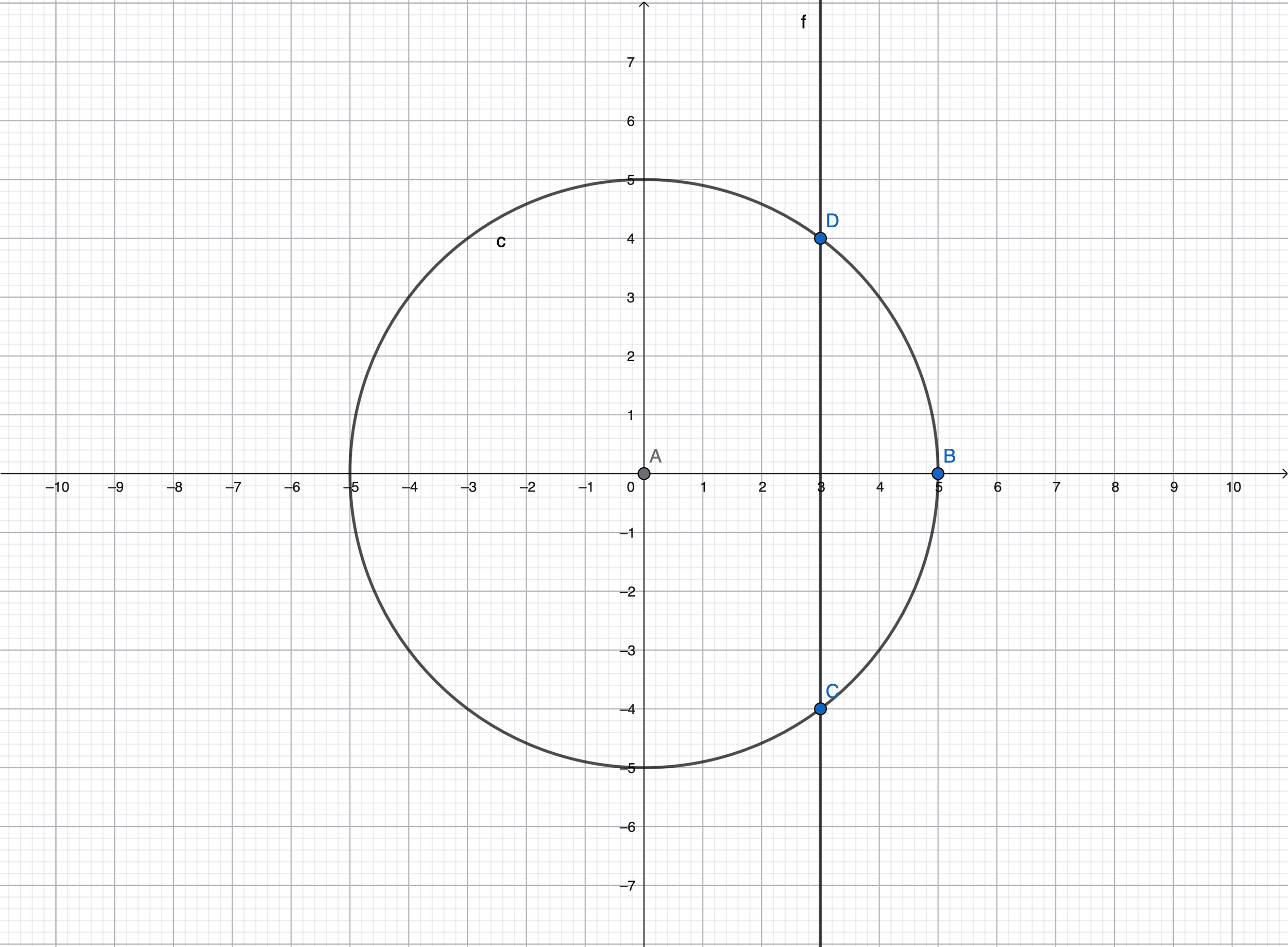
See that when x=3, y=4 and also y=-4. That’s a violation of that “only one output for each input” rule.

There is a related category of function that we can use that will allow for this sort of motion, which is good because this sort of motion actually happens! Instead of saying that y = f(x), so the input is x and the output is y, we can instead say that both x and y are some function of a third variable, called a “parameter.” Functions defined in this way are called “parametric,” and they look like this:

x = f(t)

y = g(t)

… where f(t) and g(t) are two different recipes that tell us what to do with the value of t in order to get x and y.

The clever thing about parametric functions is that the parameter, t, is not on the graph. Looking at our circle graph, we could create the same graph with the following pair of functions:

In those equations, the omega — the letter that looks like a w — is called the “angular frequency” and it is a constant that has units of 1/seconds. It’s a bit of a mathematical formalism, but the trigonometric functions need to have a pure number as an input. No units. So the angular frequency gets rid of the seconds unit and also controls the relationship between time and angle. At a later point, this will be important. For now, if this paragraph made no sense, just ignore it!

If we graphed x and y separately, with t on the horizontal axis, we would get normal, boring sine and cosine curves. There would be no violation of the vertical line test. However, when we graph x and y together, with t hidden in the background, we get a circle with radius 5 units.

To sum it up, parametric functions let us describe real world motions. In the real world, time is the controlling variable. Things happen as time passes. Time is also the hidden variable. When we look at the path an object took through space, we don’t see the time represented. If we looked at a movie, we would see time as the object actually followed the path.

The “only one output for each input” rule makes a lot of sense in this context. It literally says “you can only be in one place at a time.”

Our equation set (above) is actually parametric! Let’s look at it again to save you having to scroll up:

Notice that every variable has a subscript to indicate whether it’s an x or a y variable… except x and y themselves, of course. But t does not. There is no such thing as x-time that is different than y-time or z-time. These equations are parametric pairs that can be graphed to understand the motion of an object with constant acceleration in two dimensions.

That’s the side quest! For students who are in an advanced calculus course, and for those who go on to higher studies of physics, this stuff will become the background — the playing field, if you will — that is hiding behind almost all your later work

To Do:

• Practice Problems: OpenStax College Physics 2e problems 1, 3, 5, 11, 15, 17, 19