
You probably have most of this stuff at home anyway
1.5: Constant acceleration and the equations that go with it.
Key concepts:
Constant acceleration. In a lot of situations, the acceleration of an object is a constant value... or it's close enough for us to make the assumption that it is constant.
Algebra instead of calculus: We assume constant acceleration so that we will have equations of motion that can be solved with high school algebra. Calculus students will recognize the connections.
Recognizable graphs: Motion with constant acceleration produces a “fingerprint” set of graphs that are easy to recognize.
Textbook Section: OpenStax College Physics 2e Section 2.5
If we can assume that acceleration is constant, we can solve problems of accelerated motion using high school or college algebra without needing calculus. That’s the bottom line. As always, when we make a simplifying assumption, the key question is “can we get away with it?” — Or, putting it more politely, is this assumption accurate enough for what we need.
The short answer is yes, if we look at small segments of an object’s motion. For example, a car pulling away from a stop light is approximately constant acceleration if we ignore the point where the car is approaching the speed limit. Of course, if we can’t ignore that stuff, we will need to abandon our assumption and solve the problem with calculus, but that’s a topic for a higher level course than this one.
This section is going to be a bit math-heavy, but we’re setting up a framework that we will be using for quite a while to come, so take the time to understand it.
Let’s start with the main assumption:
This isn’t something we can put into an equation, so let’s make it a little more mathematical:
This is the physics way to say that something is constant. Whatever the current time is, the current acceleration — “a” — is equal to the initial value. Side note: You’re going to see this mathematical representation of a constant in other contexts, so make a mental note of it now!
Remember from the previous section that acceleration is the slope of a velocity vs. time graph:
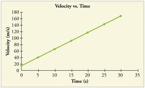
While we’re remembering things, it’s also worth remembering that these graphs are often drawn with positive slopes, like the one above. Trust me, some of them will be negative slopes, and some may even be horizontal — zero slope.
Since that graph is a line, we can use the equation of a line — y = mx + b — but with variable changes to represent the fact that:
“y” is actually velocity
“m” is acceleration
“x” is time
“b” is initial velocity
Notice that we have made another equation of motion, the same way we did in section 1.3. In this case, if we know the time, the acceleration, and the initial velocity, we can find the final velocity. Also, like all equations, we could rearrange it to solve for any variable we want.
Another side note: Somehow “delta t” became “t” and nobody said anything. Here’s the explanation:
We started with the idea of a time interval:
If we can assume that the initial time is zero, then the time interval simply equals the final time. Most of the time, this is a safe assumption, because we are usually the ones in control of the stopwatch, and we can start it whenever we want to. So we conveniently reset our stopwatch so it reads zero and we start measuring time when the interesting stuff happens.
Physics textbooks love to do a pile of algebra to show students that there is an unbroken logical chain between the equations of motion that we have learned and the equations of motion that I am about to present. If you want to see that algebra, feel free to look at it in the textbook link at the top of this page. Or, you can just trust me. If you take the two things we know so far:
… and do quite a bit of algebra with them, you get the “big four” equations of constant acceleration. I’ll present them below, before talking about what they mean.
Now, the meaning: These are equations of motion — revisit section 1.3 for a review if necessary. Like all equations, they serve two purposes:
They let us calculate stuff. If you have the values of the variables, you can solve for one that you’re missing. It doesn’t have to be the variable on the left side of the equal sign, either. If you’re willing to do the math, you can solve for any variable in the equation.
They let us understand and predict motion with constant acceleration.
A quick note: Some textbooks write equations in the usual way with decreasing exponents. Others, like the OpenStax book that this course is linked to, write their equations backwards with increasing exponents. The two notations are algebraically equivalent. Personally, I like my way as presented above. It helps students to recognize linear and quadratic equations. Again, it doesn’t matter which order you write things in as long as you don’t make an algebra mistake along the way.
Graphing motion with constant acceleration:
We have seen both position vs. time and velocity vs. time graphs so far. We’re going to add a third one: acceleration vs. time. If the acceleration is constant, this is going to be a very boring graph:
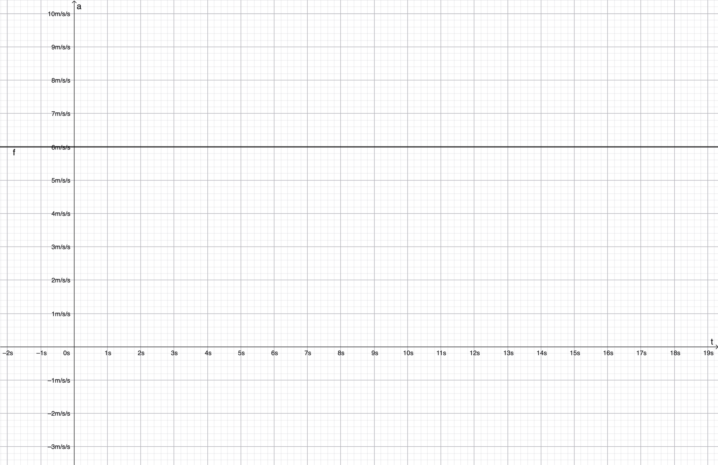
This is what the graph of a constant looks like. It’s a horizontal line, because a change in time (the “x axis”) does not change a constant!
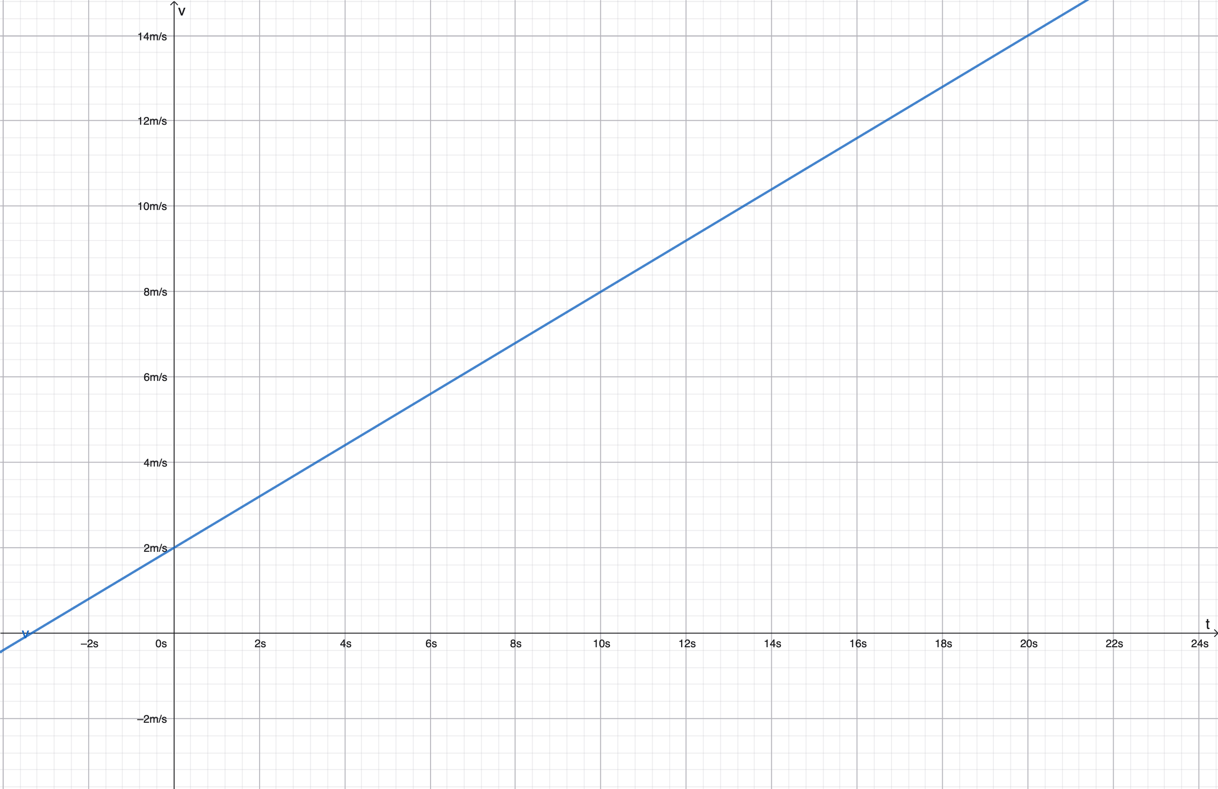
Now remember that the slope of a velocity vs. time graph is the acceleration. If the acceleration is constant, the slope of the velocity graph will be constant. In other words, we will see a straight line:
Finally, look at the third equation in the stack above. See how it is a position equation because it starts off “x=…” and also see that it has inputs of acceleration, initial velocity, and time? Looking at the exponents on the time variable, you should recognize a parabola. Here’s what the graph looks like:
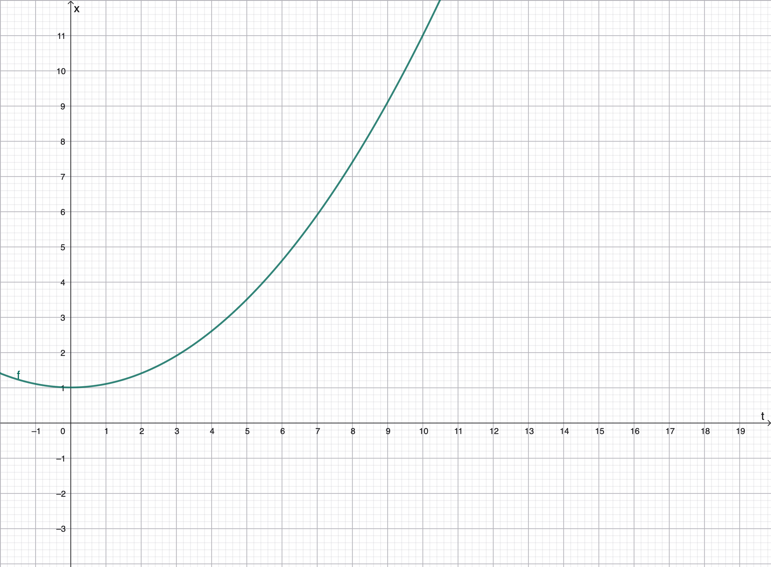
Again, physics textbooks love to present three graphs that look like this, because everyone loves positive numbers! However, there’s no reason that the acceleration could not be a negative constant. In that case, the velocity would be sloping downwards, and the position graph would be a downward opening parabola instead. These graphs are the “fingerprints” of constant acceleration. Just to review:
The acceleration vs. time graph will be a horizontal line.
The velocity vs. time graph will be a sloped line, but no curve!
The position vs. time graph will be a parabola, either upward or downward opening.
Small side quest: Negative time
Negative time does exist, and it’s much simpler than it seems. Remember, way back in the beginning of this unit, we learned that a frame of reference defines a zero point and a positive direction? For time, the positive direction is the same for everybody, but the zero point for time is under your control as you conduct the experiment. To put this in the simplest possible terms, YOU control the stopwatch. When you click the “start” button, you have defined zero time.
Negative time is just time before you clicked the start button on the stopwatch. That’s all.
One final quick note: “Deceleration”
Deceleration is a word we use a lot, and its general meaning is “slowing down.” However, we have to be more specific when we’re working with equations. Remember that velocity and acceleration are vectors. In one dimension, that means they are numbers with a positive or negative sign. "Slowing down” in this context means something very specific:
The sign of the acceleration is opposite the sign of velocity.
More often than not, a problem will have a positive initial velocity, and “deceleration” simply means a negative acceleration. However, this is not a law of nature. Check the sign of the initial velocity and give the acceleration the opposite of that sign.
Looking ahead to motion in more than one dimension, it gets slightly more complicated; however you can apply the same principle.
If an object is decelerating, the direction of acceleration is opposite the direction of velocity.
To Do:
This lab to explore constant acceleration
From textbook section 2.5: 20, 21, 23, 25, 27, 29, 33
Section Links: