
1.4 Acceleration
Make sure you feel secure in your knowledge of velocity from the previous module, because you’re going to need that foundation for what we do next.
Key Ideas:
Velocity is a vector, so the direction is an integral part of a measurement of velocity.
Acceleration is defined as the change of velocity over time.
Velocity can change because the speed changes, or because the direction changes, or because both speed and direction change. Therefore, any change in the velocity is an acceleration.
Velocity is a rate of change of position with respect to time. Acceleration is a rate of change of velocity. Therefore acceleration is a rate of change of a rate of change.
Important side quest: (Calculus concept tie-in)
Rate of change can be represented by the slope of a line. For curved lines, we can calculate average and instantaneous rates of change.
A rate of change of a rate of change can be seen as curvature of the line.
TextbookSection: 2.4 in OpenStax College Physics 2e
Acceleration is not a difficult thing to calculate. For most beginning students, the problem with acceleration is conceptual. This difficulty comes from the basic definition of acceleration: It is the change of velocity, and velocity is the change of position. In other words, acceleration is a change of a change, and that’s hard to wrap your head around.
First, a definition in words:
Acceleration = [change of velocity] / [change of time]
Acceleration has dimensions of [velocity units] / [time units] and since velocity has dimensions of [distance units] / [time units] we end up with an interesting situation: Acceleration has dimensions of
[distance units] / [time units] / [time units]
The key to recognizing an acceleration when you see one is that there will be two time units in the denominator. This may appear in a number of ways.
The most common is:
Which you may also see written as
The important thing to look for if you’re going to recognize an acceleration unit is a distance divided by two times. For example, in the US, we often report the acceleration of cars in terms of 0 to 60 mph in 6.5 seconds… or whatever the number happens to be. But look closely at that set of units. Miles (distance) per hour (time) in X seconds (time). If we wrote it mathematically, it would look like this:
… and now we can see a distance over two time units. In this case, they are not the same time unit, but that doesn’t matter. Remember that dimensions are the important things, because units can be converted to other units within the same dimension. It’s easy to make miles into meters and hours into seconds and convert miles per hour per second into meters per second per second.
The math of acceleration:
Written as an equation, acceleration looks like this
If we’re working in one dimension, that equation is enough. However, in the future when we start looking at motion in more than one dimension, be aware that each equation will split into an x copy and a y copy, which will look like this:
We won’t worry too much about 3 dimensional motion in this course, but in 3-D there would be a third copy of the equation, this time with Z subscripts.
Since this is an equation, it can be graphed, or solved for a variable, just like any other equation. If you jump back a section, you will see a graph that looks like this:

The slope of that graph is the velocity because “rise” is change of position and “run” is change of time. Remember the equation for velocity:
and compare it to the equation for acceleration:
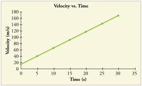
They looks similar because they are both slope equations. Acceleration is the change of position (rise) over the change of time (run). If we look at a graph of velocity vs. time, we can find acceleration as a slope:
Side quest: Average vs. Instantaneous rates of change:
Physics teachers love to present the graphs that I presented above, because it makes everything look simple. In reality, these graphs would not be straight lines. While this makes the math a little more difficult, it does not change the basic idea. Velocity and acceleration are slopes and even a curved line has a slope. The only difference is that the slope of a curved line is changing.
For both types of graph, we can still describe a “slope” even when the graph is a curve. There are two ways we can do this:
Average Velocity: Pick two points on the curve that are relatively close to each other and draw a straight line between them. Figure out the slope of that line.
Instantaneous Velocity: Pick a single point and draw a tangent line. Figure out the slope of that line.
Let’s look at these two ideas. As we look at graphs, look very carefully at the vertical axis label! Position graphs will give us velocity, and velocity graphs will give us acceleration.
Average Velocity: Pick two points and make a line out of them. Look at this graph of position vs. time:
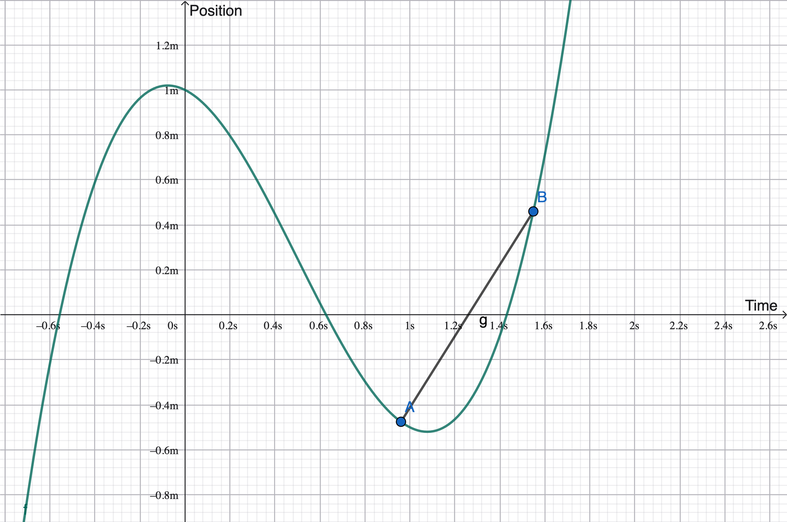
The position vs time graph is obviously not a straight line. I chose two points on the graph, labeled A and B, and drew a straight line between them. I could find the slope of that line easily, by using a standard rise over run slope calculation.
Notice that the actual object does not travel in a straight line from A to B. Whatever slope we calculate from that straight line will only be an approximation of the actual motion. We are, in fact “averaging out” the curve, and the slope we calculate from this straight line segment will be an average velocity.
Instantaneous Velocity: Pick a point and draw a tangent line. Find the slope of that tangent line. Look at the same graph, below, but in this case, I have put a tangent line at point C.
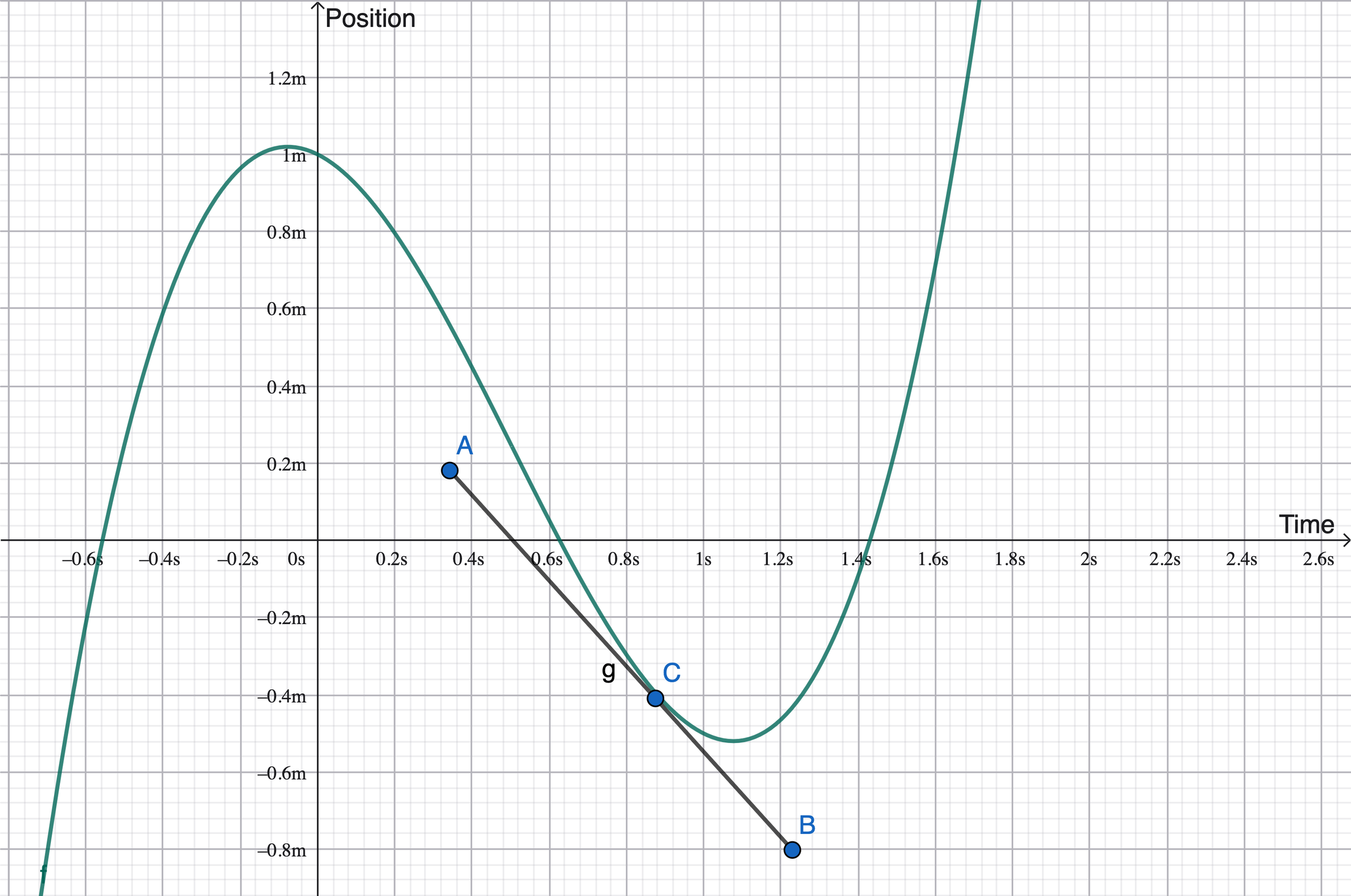
We can still calculate a slope. Either we use a couple of convenient points (A and B) and calculate rise over run, or we use a calculus technique called a derivative. Either way, we will get a slope. Regardless of how we calculate it, the slope at point C is the slope of that tangent line. It is the slope at an the instant the object passes through point C, so it’s called an instantaneous velocity.
We can use exactly the same mathematical techniques to calculate accelerations. We just have to start from a velocity vs. time graph instead of a position vs. time graph. If we do these calculations, we get average and instantaneous accelerations instead of velocities.
Side quest: The meaning of curvature
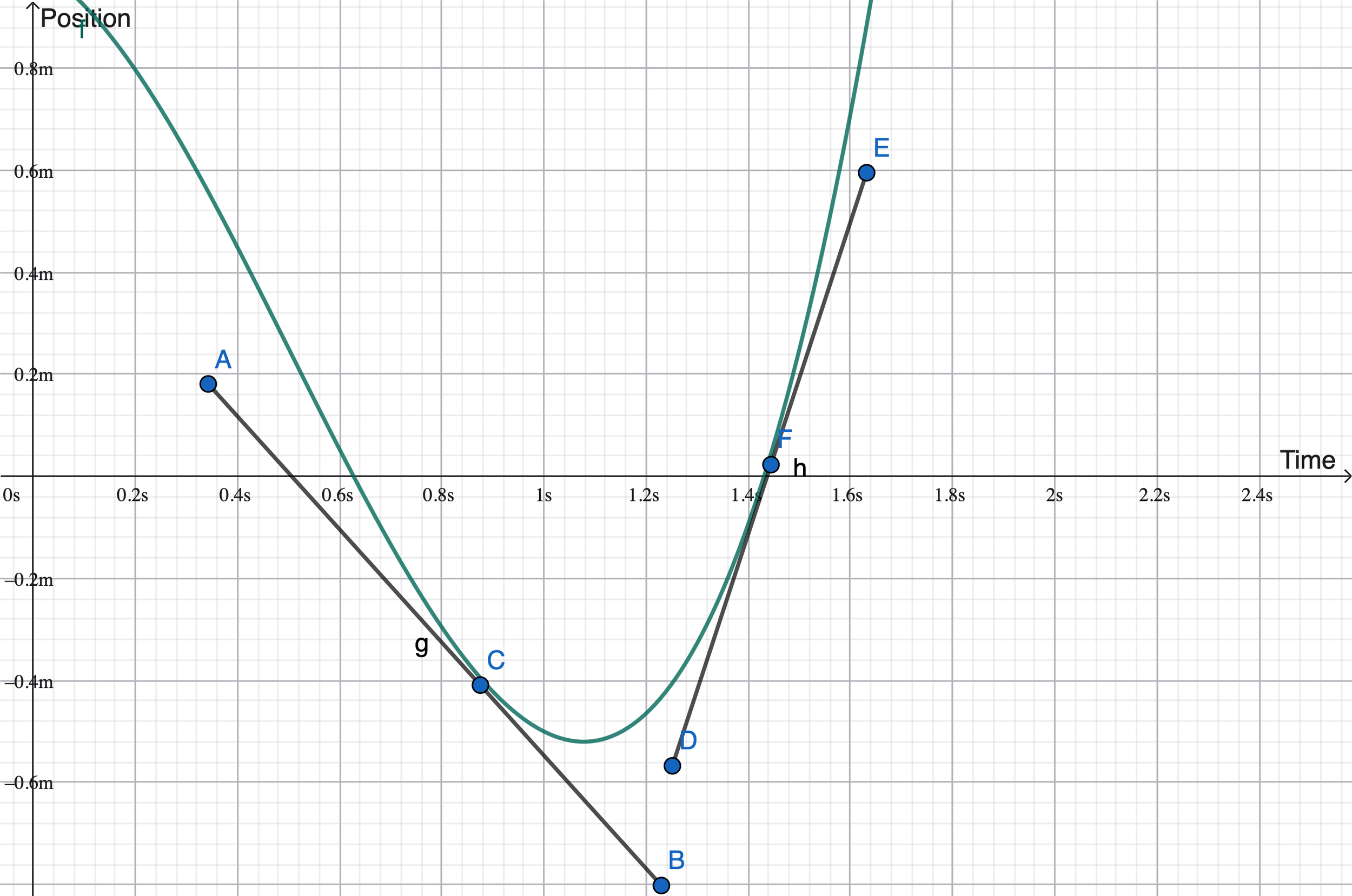
Let’s take that same instantaneous velocity graph that I just created, but this time, I’m going to add a second tangent line:
The graph was getting crowded, so I zoomed in on it a bit to make the tangent lines more visible. Remember that this is a position vs. time graph so the slopes of those tangent lines give us two different instantaneous velocities.
The slope of line AB gives us the velocity at the instant the object is at point C
The slope of line DE gives us the velocity at the instant the object is a point F
We have two velocities and there is a time interval between them. Using the acceleration equation, we could calculate the acceleration between points C and F.
Now let’s go through a few logical steps:
The slopes of the tangent lines give us velocities at the tangent points.
The tighter the curve of the position graph between the two tangent lines, the more the velocities will change between the two tangent points.
The more the velocities change, the bigger the acceleration.
Putting it all together, on a position vs time graph, acceleration is visible as the curvature of the graph.
Now let’s use the same logic in reverse:
A straight line graph has zero curvature
A straight position vs. time graph has zero acceleration.
What does curvature mean on a velocity vs. time graph? Start by remembering that the slope (average or instantaneous) of a velocity graph is acceleration.
If the velocity vs. time graph is a straight line, the acceleration is not changing.
If the velocity vs. time graph has curvature, the acceleration is changing.
Changing acceleration is a perfectly normal thing, but it is a bit beyond the scope of an introductory physics course. Other than mentioning it here, we won’t worry about it.
A few odds and ends:
Introductory students often get confused about finding instantaneous velocity when the graph is a straight line. If the graph does not curve, or if a segment of a graph is a straight line, the velocity is the same everywhere on that segment. So the instantaneous velocity is the same as the average velocity, which is the same as the slope of the segment. The same is true when calculating accelerations from velocity vs. time graphs.
Wow, that was a lot…
To do:
Try problems
No lab yet. There will be one in the next section.